
Modeling Causal Relationships
As we saw in the previous post, circumstances faced by the Baltimore Ravens’ Lamar Jackson and Tyler Huntley could have contributed materially to their differences in observed performance. Consequently, comparisons of stats on a per-play basis could potentially be misleading.
Given that we know how one quarterback performed, we’d love the ability to peer into the mirror universe where the other quarterback was playing in the same exact play instead (aka the counterfactual), and just compare performance for each over a decent set of plays. Not too many Dr. Stranges to generate that sort of thing around though, so concern over whether other factors are confounding the patterns we observe remains ever-present in an observational data setting. Luckily, there are statistical techniques that can at least get us closer to that hypothetical scenario.
Let’s take another look at all the plays from 2021-2022 from Lamar Jackson or Tyler Huntley, this time focusing on those had a direct hand in (QB dropbacks & intentional QB runs). The data from nflverse R packages also graciously provides information on a number of additional factors. A list of possibly influential factors might include:
- field position
- homefield advantage
- down and distance
- time remaining
- expected pass likelihood
- expected win likelihood (trailing or leading, etc.)
- offensive personnel
- offensive formation
- defensive personnel
- opponent defensive strength (collected independently from Football Outsiders)
- offensive playcall
- point in the season
- season
- stadium roof
Direct QB Effect Model
One’s first instinct could be to assemble a predictive model using all these possible influences, including who was playing quarterback. NFLverse data delivers at least some information on each of these play characteristics. Machine learning, fueled with enough data and some computing power behind it, is typically quite skilled at this task. We could then combine all the model predictions for Jackson as QB and Huntley as QB, and compare them to see how much better one would be expected to perform over the other on average.
The problem is that these predictive models are typically built to use any data its fed to predict the outcome, expected points added (EPA) for our use case, without any understanding of how they might be linked in terms of cause and effect. To use the correlations observed in these models for decision-making, without understanding of how they are linked in a causal pathway, can easily overestimate or underestimate cause-effect relationships, or potentially hallucinate ones that don’t even exist. The borderline silly but easily understandable example is that a model given a lot of game information could easily detect high correlation between 4th quarter kneel downs and winning the game. But converting that finding into advice to kneel down late in games regardless of situation would be obvious malpractice.
This is where causal inference techniques come in. Randomized trials are typically the gold standard, but an experiment where we randomly swap the two quarterbacks on a play-by-play basis for a season is probably a tough sell to the Ravens organization. Luckily, different fields have developed techniques to try and parse out the magnitude of causal relationships, should they exist, in observational data. What we will need is a conceptualization of how different factors relate sequentially in order to point these models in the right direction. I’ll make an attempt at one here, with some background knowledge and some guidance from whose who have tackled the question previously.
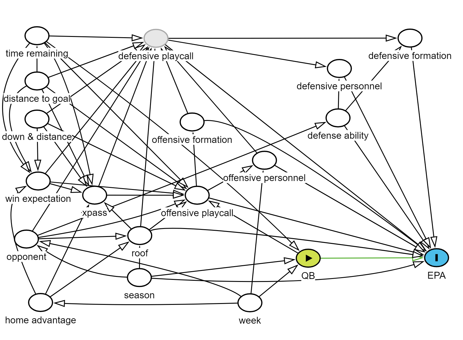
There are upstream temporal factors that might impact the likelihood of a specific QB being in the game: time remaining (as a backup, Tyler Huntley would be inserted as an injury replacement later in games), week (a serious injury to Lamar Jackson would lead to consecutive weeks Huntley was playing), and season (Jackson might have been more injured in one season than the other). Those are possible confounders which likely need to be adjusted for to avoid bias, though no colliders that would induce bias if put into the model. Still, there are other play characteristics we identified could be strong influence on success. Accounting for them our model could enhance its predictive value, as long as we don’t absolutely inundate our model with things to consider. If we control for important influences, we should be able to gauge the direct impact of the QB on success.
The estimation technique I’d like to take out for a spin here is a causal forest. I won’t get into it too deeply here, but it is a nicely specialized tool and a potent one for this purpose because of some characteristics that other methods might lack:
On a basic level, its focus is on the predictor, so it’s designed to reduce the bias and error around any estimate of the difference between the two options.
It leverages modern computing power via machine learning to blend different statistical models (such as a number of different tree-based models) and create more accurate predictions, resulting in causal estimates of effect that are fairly consistent.
This implementation can use crossfitting to make predictions of standard errors using data not used to fit the model.
It can account for some game-level factors we might not have the ability to explicitly account for in our model to provide more accurate uncertainty around our estimate.
It works well in concert with augmented inverse propensity weighting (AIPW) which is doubly robust, meaning as long as we can predict either the likelihood of our predictor or our outcome, it should produce stable and valid results.
Now, let’s run the model with the above variable adjustments and estimate the impact of one of the Ravens’ quarterbacks compared to the other. To help the model out, we’ll try to minimize the noise by focusing on plays where the QB should have a direct effect, dropbacks and intended QB runs.
- down (categorical, one-hot encoded)
- ydstogo
- yardline_100
- posteam_type
- game_seconds_remaining
- xpass
- wp
- roof
- defteam (categorical, one-hot encoded)
- offense_formation
- offensive personnel (categorical, classified by number of linemen and TE/RB using participation data)
- defenders_in_box
- defense personnel (categorical, classified by number of defense backs using participation data)
- play_type (categorical)
- Rush.DVOA (via Football Outsiders)
- Pass.DVOA (via Football Outsiders)
- season
- week
| Estimate | 95% LCL | 95% UCL | |
|---|---|---|---|
| Average EPA Difference (Jackson -> Huntley) |
-0.220 | -0.313 | -0.127 |
Implementing our causal forest model with all these predictors and applying the AIPW estimator, our model estimates that average EPA per play drops about 0.22 when Huntley is in for Jackson (See Table 1), a fair bit larger than the 0.08 difference seen using established model tallies. To put that into perspective, according to 2022 QB stats for all games played from rbsdm.com, that tradeoff is in the ballpark of swapping out Dak Prescott’s per play efficiency for that of Russell Wilson’s first ride with the Broncos.
Total QB Effect Model
Having said that, a concern arises from including so many factors in a causal inference model. For example, it’s likely that Lamar Jackson running ability influences the defensive personnel the opposition puts on the field, and that may impact the resulting EPA, similar to in this example. Adjusting for that would likely lead to underestimating the ways in which Lamar’s presence improves offensive production. We’ll use our directed acyclic graph to adjust the model to include those indirect pathways.
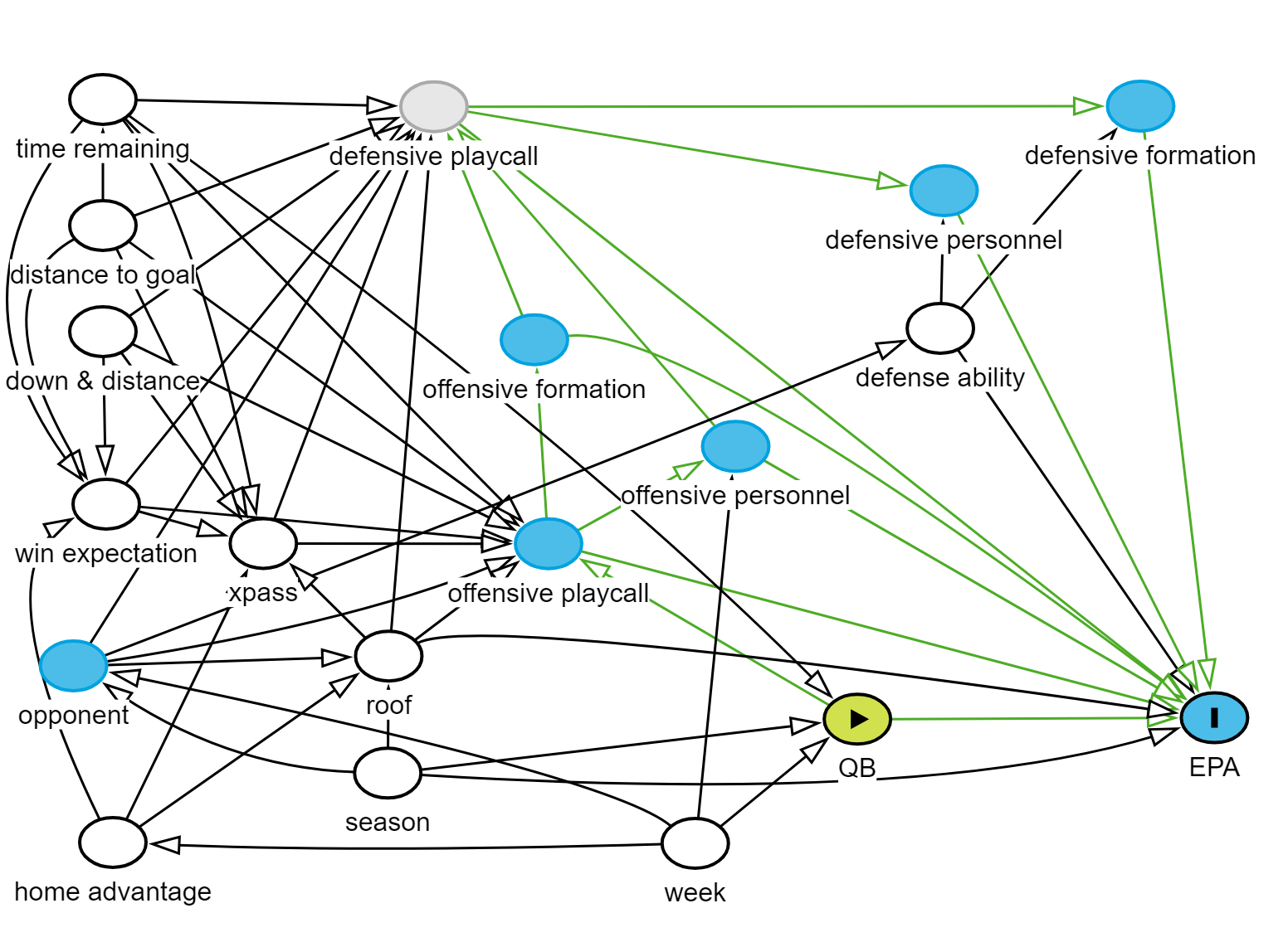
Setting up the model to be more permissive about different ways the QB can influence EPA leaves us with much fewer components for which we need to adjust. The paths to play success that we don’t want to block off are marked in green on the diagram. Here, we’ll limit adjustments to situational factors that drive playcalling on both sides of the ball:
- down and distance
- distance to end zone
- gametime remaining
- win likelihood
- home or road game
- expected pass rate
- week
- season
- stadium roof
- opponent defensive aptitude
- down (categorical, one-hot encoded)
- ydstogo
- yardline_100
- posteam_type
- game_seconds_remaining
- xpass
- wp
- roof
- Rush.DVOA
- Pass.DVOA
- season
- week
| Estimate | 95% LCL | 95% UCL | |
|---|---|---|---|
| Average EPA Difference (Jackson -> Huntley) |
-0.242 | -0.339 | -0.145 |
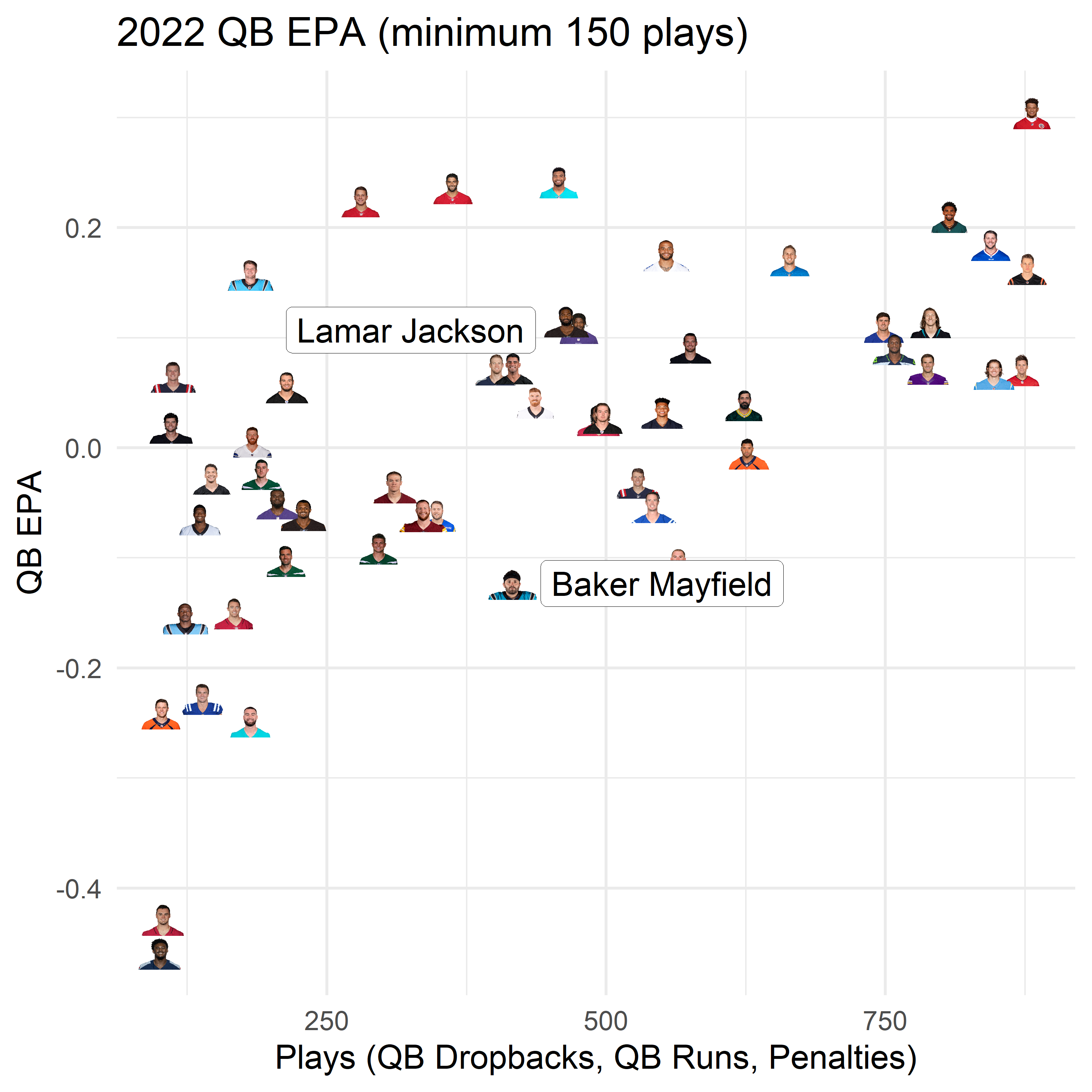
This model predicts a slightly greater disadvantage when we allow for more pathways to influence the QB relationship on play outcome, albeit not by much (Table 2). Depending on your preference, we have a statistical conceptualization of how influential Lamar Jackson’s presence is compared to his understudy. That difference, when mapped over average QB EPA from the 2022 season, would be comparable to dropping from Lamar Jackson’s efficiency (#11) to slightly worse than Baker Mayfield’s (#45).
So our model is certainly arguing that Lamar Jackson’s presence was probably even more underrated than raw statistics would indicate, and his value over the Ravens’ current replacement option is substantial. The magnitude of that actually sounds pretty harsh, but there’s some uncertainty around that estimate. There’s also the caveat that the offensive coordinator responsible for the playcalling, Greg Roman, stepped down, so the degree to which this expectation changes with Todd Monken piloting the ship is hard to declare reliably.
Strategic QB Deployment?
Now, causal forests are built in particular to investigate how different our variable of interest acts on different subsets of the data. Now, in our data, QB choice is dictated by injury, but at the times when both would be available, we could ask if there are circumstances where we would want to use one option versus the other. Are there instances where the model would strongly recommend subbing in Huntley for Jackson? For fun, let’s check with a bit of help from the policytree package.
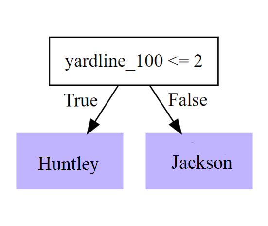
Limiting it to splitting our plays up based on one variable results in a curious recommendation. There are only a paltry 18 instances in our set of plays where they ran plays from the 2 yardline or closer, 15 for Jackson and 3 for Huntley. But the raw data does show Jackson as noticeably worse than Huntley at that distance (avg QB epa = -0.9 for Jackson; 0.9 for Huntley). The model predicts a closer split (avg QB epa = -0.82 for Jackson; 0.15 for Huntley). Not sure I’d take it up on that advice, given our outlier cleanup (and I might specifically advise against any leap-over-the-line attempts for Huntley should the distance be closer to 2 yards than not). But there’s a small chance it’d be worth revisiting playcalling for Jackson in near goal situations to find adjustments and increase success.
Another interesting split, albeit based on not much more data (39 plays), is for 4th down. Given the ball on 4th down, Huntley is expected to produce, on average, 0.39 EPA than Jackson. This is compared to the -0.26 EPA expected when he’s involved on downs 1 through 3. A deeper dive into how those circumstances differ might be fruitful.
| Estimate | Std. Err | |
|---|---|---|
| 1st down | -0.183 | 0.064 |
| 2nd down | -0.340 | 0.104 |
| 3rd down | -0.269 | 0.114 |
| 4th down | 0.390 | 0.695 |
Run Game Effects?
There may be less than 700 running plays over the two seasons being observed, but we can still run through the same process to see our model can detect a difference. As a reminder, the raw observed difference in EPA on run plays was around 0.04 in favor of Huntley.
| Estimate | 95% LCL | 95% UCL | |
|---|---|---|---|
| Average EPA Difference (Direct Effect) | 0.031 | -0.104 | 0.166 |
| Average EPA Difference (Total Effect) | 0.043 | -0.085 | 0.171 |
So, while there’s certainly some thought that running quarterbacks manufacture indecision in would-be tacklers and makes it easier for an accompanying running back to produce, it’s not something that this model is picking up for these two specific quarterbacks. Of course, it may be that while Lamar Jackson is known to be a dynamic runner, Huntley also has some speed and is not regarded as a slouch in that category by opponents.